
Modeling Shifts in Reversible Chemical Reactions and Economic Markets
Abstract
The purpose of this paper was to investigate how economic principles of supply and demand can model reversible reaction’s equilibrium, using computational approaches. This study primarily utilized the WebMO server, Gaussian software, and Mathematica-based modeling to simulate two key reversible reactions: and . By adjusting different components of these reactions, such as their reactant and product concentrations, temperatures, and perturbations, the behavior of each system was cross-applied to analyze effects on economic markets. The results suggest that increases in reactant concentrations resulted in proportional increases in product formation, which mirror market responses to supply boosts in a given situation. Additionally, perturbations, such as sudden changes in reactant concentrations, caused the system to shift dynamically and restored balance within the chemistry and economics-based models. Ultimately, integrating economic and chemical models through interdisciplinary pathways allowed for the opportunity to further refine the computational analogies through more complex reactions.
Introduction
Establishing an equilibrium in various disciplines, such as chemistry and economics, is important to create a balanced system. In chemistry, equilibrium refers to a reversible reaction where the products react to form the original reactants at equal rates Shaymardanov et al., 2022. Essentially, this means that the rate of the forward reaction equals the rate of the reverse reaction. The equilibrium constant, , describes the balance between reactants and products at equilibrium. This constant is extremely important when determining how a system at equilibrium will adjust if it is disturbed, disequilibrium. Additionally, the Gibbs free energy of a reaction is imperative in accurately determining whether a system is at equilibrium. Gibbs free energy measures the available energy in a system (or the change in energy of a system) using enthalpy, entropy, and temperature. Gibbs free energy helps determine whether a reaction will proceed spontaneously under the given conditions Middelburg, 2024.
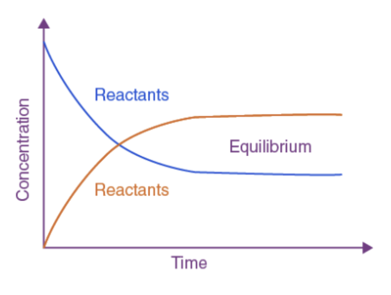
Figure 1:Chemical Equilibrium
Another key principle this paper hinges on is Le Chatelier’s principle. Le Chatelier’s principle is incredibly important in predicting how a system will respond and restore equilibrium. Essentially, Le Chatelier’s principle states that if an external change affects the equilibrium, the position of equilibrium must shift to counteract and re-establish an equilibrium Peris, 2021. The products and reactants have reached equilibrium where the concentration stays relatively constant Figure 1. Although the minuscule shifts between products to reactants are not visible in most graphs, reversible reactions’ dynamic nature assumes the products and reactants are always reacting with each other to re-establish equilibrium Figure 1. When the equilibrium shifts and responds to the stress, it must shift in the direction that will minimize the stress applied to a system. Different stresses, such as shifts in temperature, concentration, or pressure, may force an equilibrium to shift either in the opposite direction, to offset the change, or in the same direction, to reduce the added stress. Ultimately, Le Chatelier’s principle explains how a reaction will dynamically adjust to external changes.
In economics, equilibrium is also established in a similar manner. Within a simplified market of supply and demand, the price of a good and its quantity must be balanced when an exchange takes place.
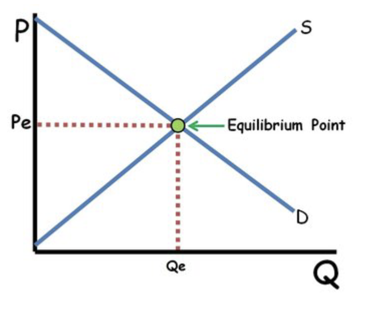
Figure 2:Supply and Demand Graph
The intersection of an upward-sloping supply curve and a downward-sloping demand curve is called the equilibrium, which is a point specified at a certain price and quantity Figure 2. The supply and demand curves can be shifted due to a multitude of factors Perkis, 2021. Supply can shift due to a change in the price of resources, the number of producers, improvements in technology, fluctuations in taxes or subsidies, and influences on consumer expectations. On the other hand, demand can shift due to differences in tastes and preferences, the number of consumers, changes in the price of related goods, fluctuations in income, and influences on consumers’ future expectations.
Similar to chemistry, equilibrium in economics follows a dynamic nature, constantly adjusting to different external factors such as resource costs, subsidies, and government regulations Jordan-Wood, 2024. The price of a certain good is what drives markets towards balance, similar to how Gibbs free energy establishes equilibrium in chemical systems.
Although the connections between chemistry and economics may not be immediately apparent, this paper aims to research possible and existing parallels at a deeper level. Both, chemistry and economics, involve systems that seek balance through opposing forces. For instance, in a chemical reaction, the concentrations of reactants and products adjust based on external factors to re-establish equilibrium. On the other hand, in an economic market, prices adjust to shifts in supply or demand to efficiently reallocate resources.
To further analyze overlapping trends between chemistry and economics, a few key assumptions were made. First, the reactants are compared to the supply curve. In a practical chemistry context, this means that an increase in reactants pushes the reaction towards producing more products. In a practical economics context, this means that increasing the supply pushes the market towards lowering the equilibrium price. Second, in a similar manner, the products are compared to the demand curve. Third, the equilibrium constant, , is compared to price elasticity of demand. Price elasticity measures the change in the demand for a product as a result of a change in its price Jordan-Wood, 2024.
If the demand for a product is elastic, a small change in price leads to a significant change in quantity demanded. Conversely, if the demand for a product is inelastic, a change in price leads to a small change in quantity demanded Jordan-Wood, 2024. Essentially, the elasticity of demand measures the sensitivity or responsiveness of the quantity demanded to changes in a product’s price. This economic principle corresponds with the equilibrium constant because they both compare smaller changes to evaluate larger systems. Finally, perturbations in chemical systems can be compared to shocks in economic conditions Farrell & Ioannou, 2000. As explained previously, external influences can shift the balance and automatically adjust a system. In context, altering temperatures in a chemical system will be compared to the effects of increasing tax rates in a market.
These four assumptions set up the basis of this paper’s purpose, which is to answer the following question: How can shifts in reactant or product concentration (in a reversible reaction) be modeled similarly to market supply and demand shifts?
Computational Approach
To maximize the result’s validity, two unique models were created for two specific reactions. The first reaction is the following acid-base reaction: . This reversible reaction’s properties accurately align with the concept of market equilibrium in economics. This reaction sets up the model’s key components so that they can be cross-applied to additional reactions. The second reaction is the dimerization of nitrogen dioxide: . This was chosen because the equilibrium constant of this reaction is solely dependent on the concentrations of the reactants and has a corresponding influence on economic equilibrium calculations Romero & Rossano, 2019.
These two reactions were run through a WebMO Schmidt, 2007The North Carolina High School Computational Chemistry Server, 2024, a computational chemistry platform that specializes in outputting molecular properties using quantum chemistry software, such as MOPAC and Gaussian.
In order for these reactions to be accurately run in WebMO, a “Geometry Optimization” job must be run. This enables WebMO to find the most stable arrangement of atoms in a given molecule, which means minimizing the molecule’s total energy. To run this job, in the WebMO Job Manager page, a “New Job” is created. Then, the molecule is built using the “Build” tool, and the geometry is optimized using the Gaussian computational engine. Gaussian Gaussian, 2024 was used for all the molecules chosen because this paper only focuses on smaller molecules and Gaussian is more suitable for precisely calculating smaller molecules’ geometries and energetics. Then, the B3LYP theory is chosen (under the DFT umbrella) with a basis set of 6-31G(d) for all molecules except for and . This is because and have a more complex atomic arrangement, so an accurate basis set of 6-311+G(2d,p) will produce more precise results. A total of six “Geometry Optimization” jobs were run.
Because is a water based reaction, a solvent model calculation is included. This allows the calculation to simulate the effect of water as a solvent, which allows WebMO to calculate the energetics of the reaction system more accurately.
To calculate the actual data in each of these molecules, a “Vibrational Frequency” calculation is run for each of the six molecules. This allows for thermodynamic properties to be calculated for each molecule, which provide further insight into a molecule’s properties. Specifically, the Gibbs Free Energy and Enthalpy values are used for each molecule to create a reaction-specific model.
After all the data was collected, two models were built in Wolfram Mathematica. Mathematica is a powerful computing software that is most commonly used to solve and model complex problems from various disciplines. For the purposes of this paper, Mathematica was used to create a model that demonstrates chemical shifts in economic contexts.
In a new Mathematica notebook, the gas constant, the Gibbs free energy constant, and the Hartrees to Joules per mole conversion are established at the beginning of each model. It is also important to note that most of the code for both models is the same, except for the specific data (in constants) different between both reactions. The gas constant, in Joules per mole per Kelvin, was defined, and will be used in thermodynamic calculations. The conversion from Hartrees to Joules is also established to keep all calculations in the same unit. Then, the Gibbs free energy for each molecule is calculated by converting the Gibbs free energy from Hartrees to Joules per mole. To calculate the change in Gibbs free energy, based on the changes in temperature, a function for each molecule is defined. Then, to convert the change Gibbs free energy to the equilibrium constant , “theDeltaGtoK” function is created that expresses the following equation: .
Next, the “RateConstants” function is created to calculate the forward rate constant, , and the reverse rate constant, , for a reaction based on the equilibrium constant, . This sets up a formula for the differential equations that will be calculated. Then, to establish a reaction’s equilibrium, the “ReactionEquilibrium” function is defined, which models the time evolution of the reactants and products. This function also initializes a few local variables for the differentials equations. The inputs for the differential equation are written concisely (before their calculation) with the “dReactants” and “dProducts” variables, which define the rate of change for the reactants and products, respectively. Finally, a system of differential equations is created, where r[t] and p[t] represent the concentrations of the reactants and products at a specific time, t.
After establishing the basic chemistry, the model focuses on the economics approach. First, an “EconomicDynamics” function is defined, which models an economic market’s supply and demand dynamics in context. The local variables, including “Supply”, “Demand”, “Elasticity”, and “EquilibriumPrice” are also initialized. Afterwards, each of the four assumptions are coded into the model. The equation for elasticity is scaled by a factor of 10 to see its influence on the model when compared with the reversible reactions.
Next, the interactive model is created with the “Manipulate” command, which initializes the different plots that will be created and the variables required to create them. Then, the equilibrium constant is calculated based on the current temperature, defined as “Temp”, using the previously coded function “DeltaGtoK”.
Afterwards, the perturbations that would influence an economic market in a chemistry context are established with the current concentrations of the reactants and products and the calculated rate constants. In the way that the chemistry results were portrayed, the economic dynamics with perturbations included are also calculated with the “EconomicDynamics” function.
Then, a plot for the concentration of reactants and products over time, called “ChemPlot”, is generated based off of the current products and reactants calculated. Similarly, a plot for the supply and demand curves, as a function of price, is generated based off of the economic results. Finally, different ranges of values are established for the reactants, products, perturbations, and temperature (in Kelvin).
Ultimately, the two models created accurately portray the dynamic equilibrium between and and compare them to their associated economic-based supply and demand system. Because of the equilibrium constant, the chemical and economic dynamics are modeled in a manner that creates an interactive simulation. Using the “Manipulate” command, it is possible to change the concentrations, perturbations, or temperature each reaction takes place at, and see the respective influence on the supply and demand curves.
Results
At its pre-condition representation, the model for and for outputs a simple economics graph. First, the sliders representing the model in a chemistry context are demonstrated below Figure 3. Second, the basic chemistry model demonstrates the reactants’ concentration, products’ concentration, and equilibrium point Figure 4. Third, the basic economics model with a supply curve, demand curve, and equilibrium point (if an intersection occurs in the defined range) is shown.
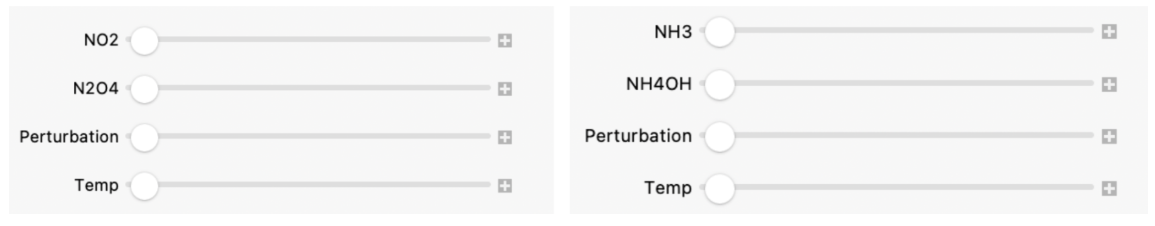
Figure 3:Sliders for Chemistry Aspects in Both Interactive Models
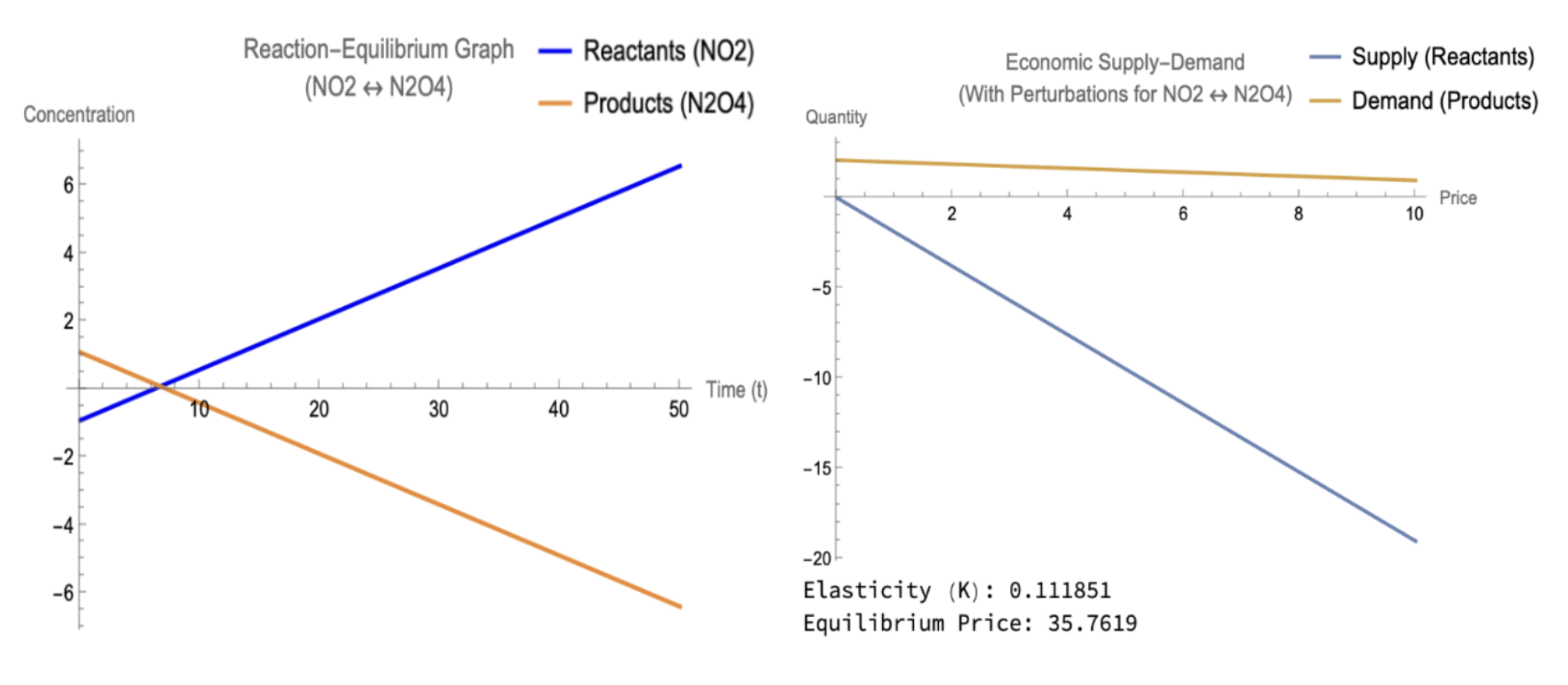
Figure 4:Base Chemistry and Economics Models
Essentially, base_models shows how the model would output an economic graph with quantities of 0 for the reactants and products. The economic graph measures prices vs. quantity, which will be the same format followed for all additional economic graphs in this paper.
To explain the validity of the results, different economic scenarios will also be discussed and explained alongside the chemistry systems. First, when reactant was introduced into the system with no initial products, over time, began converting into . This can be seen in Figure 5, specifically at the chemical equilibrium. Although the forward reaction seemed to dominate the reaction initially, as the system approached equilibrium, the rate of the reverse reaction also increased, which stabilized the concentrations. From an economics standpoint, these results correspond to a market with a sudden influx of supply. The supply curve shifted to the right substantially, which lead to a decrease in the equilibrium price in the short-term. In the long-term, the market adjusted as the demand rose to counteract the supply influx.
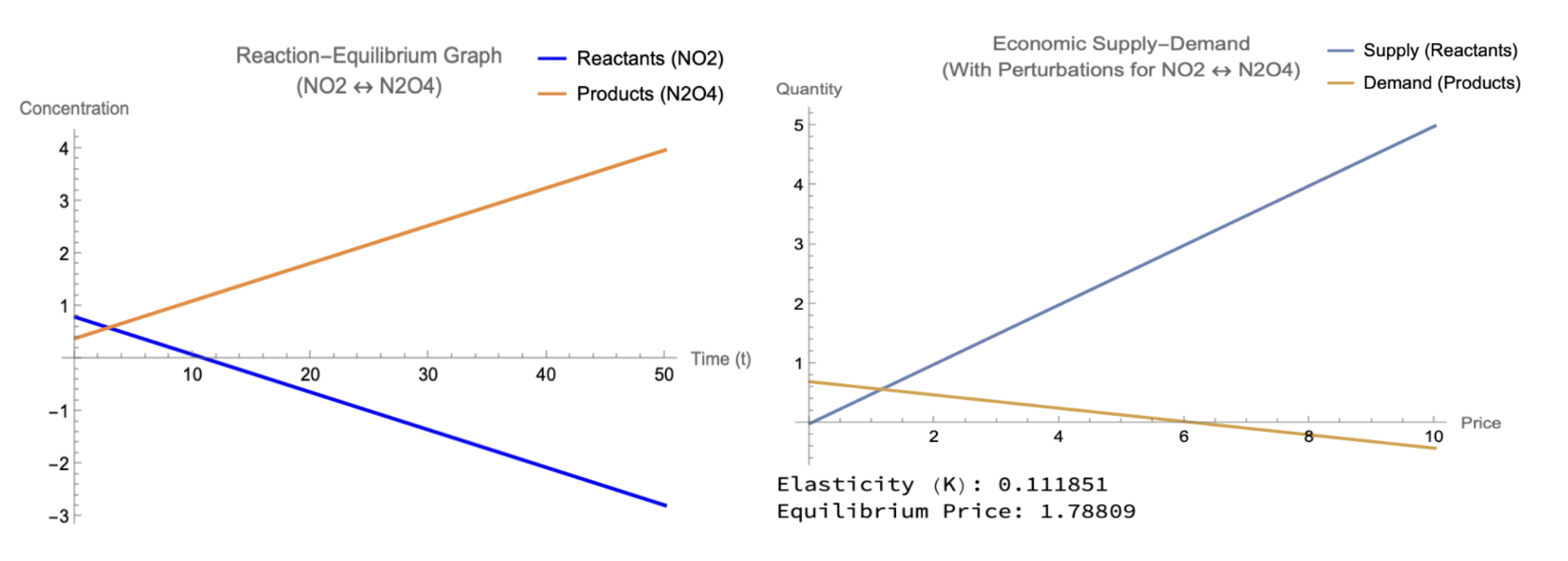
Figure 5:Reactants Introduced in Chemistry and Economics Models
Next, with the reactant present in the system, a negative perturbation was applied to the concentration of Figure 6. This reduced the available reactants mid-reaction. The concentrations dropped sharply and the forward reaction slowed. This difference can be seen between the equilibrium constant, , in the addition of reactants to the addition of a negative perturbation. In an economic context, this market can represent the impacts of a supply chain shock. A sudden decrease in the supply curve may have been caused by external factors, such as resource shortages or logical disruptions. The leftward shift of the supply curve increased the equilibrium price in the short-term, which would decrease the quantity demanded at the specific equilibrium point. However, the demand curve itself remains unaffected, which shows that the elasticity of this market is relatively inelastic, as consumer interest continues despite a lower supply and higher market price.
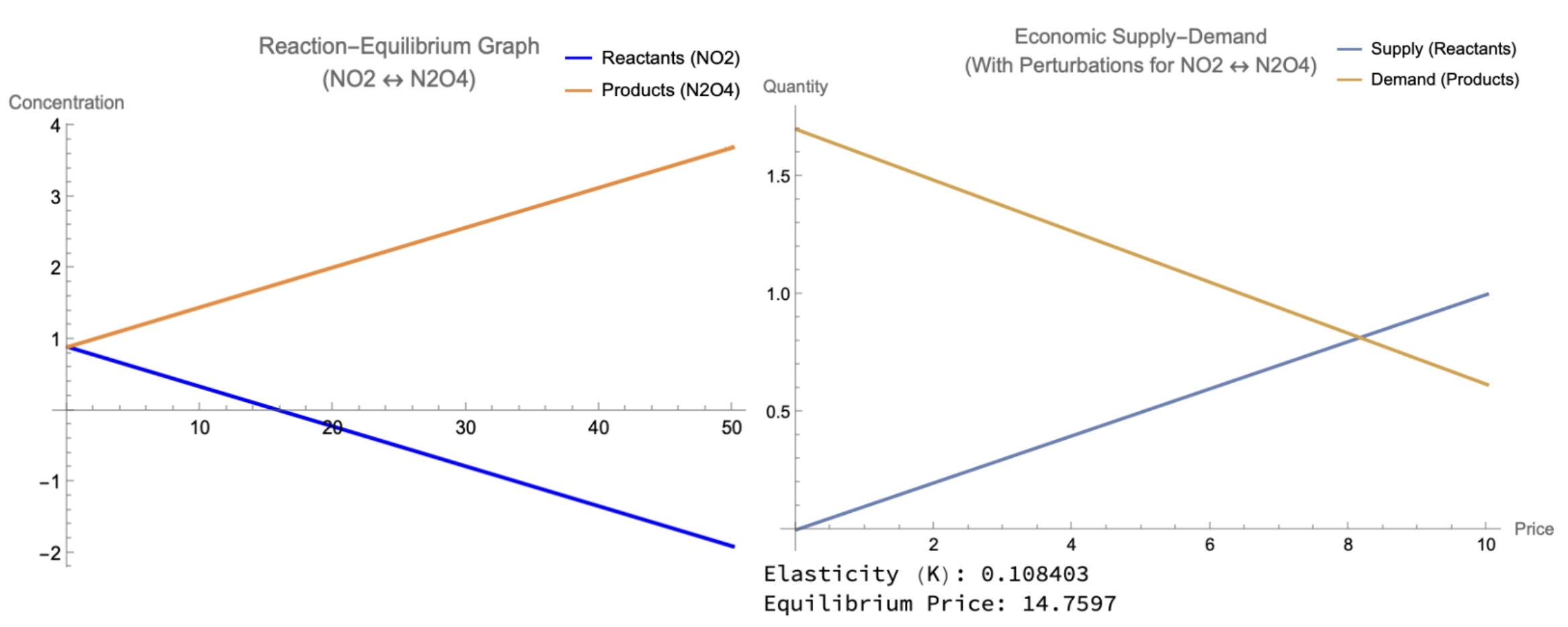
Figure 6:Reactants and Negative Perturbations on Chemistry and Economics Models
In Figure 7, the products, , were artificially introduced mid-reaction to create a response in the economic market. This demonstrates the chemical system’s response, where concentrations significantly increased temporarily. This caused the reverse reaction to accelerate, as seen with the value, and converted some of the back into . From an economic standpoint, this situation represents a substantial surge in demand. In the real world, this can be seen during the holiday shopping season, where consumers significantly increase their spending. This resulted in the demand curve shifting to the right, which increased the equilibrium price and simultaneously simulated supply-side responses.
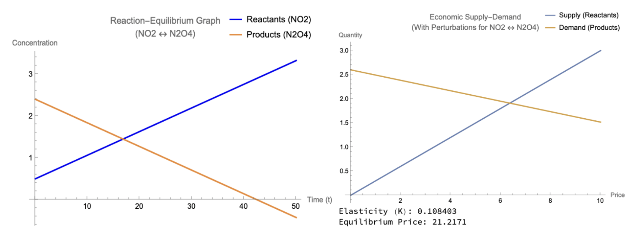
Figure 7:Reactants, Products, & Negative Perturbation on Chemistry and Economics Models
Finally, Figure 8 demonstrates that although equal concentrations of and were inputted into the model, these were not remotely close to the correct concentrations for this system to attain the equilibrium. Within this system, the equilibrium constant indicates that product formation is incredibly limited because the reactants were not given substantial concentrations or time frames to convert into products. However, in an economic context, a clear equilibrium point exists, with the demand curve following more elastic properties than the supply curve Figure 8. This means that the supply curve continues to decrease as resources be used and eventually deplete; contrastingly, the rising demand curve reflects a continuous increase in product consumption. Specifically, the low elasticity and relatively high equilibrium price demonstrate a constrained market that functions with a high demand and relatively limited adaptability. In the real world, this could be seen where would represent the supply of a raw material, while would represent the demand of a processed good. This model’s economic implications are unique, as they demonstrate that due to the equilibrium price’s elevated level, the scarcity of raw materials and increasing production costs are directly seen.
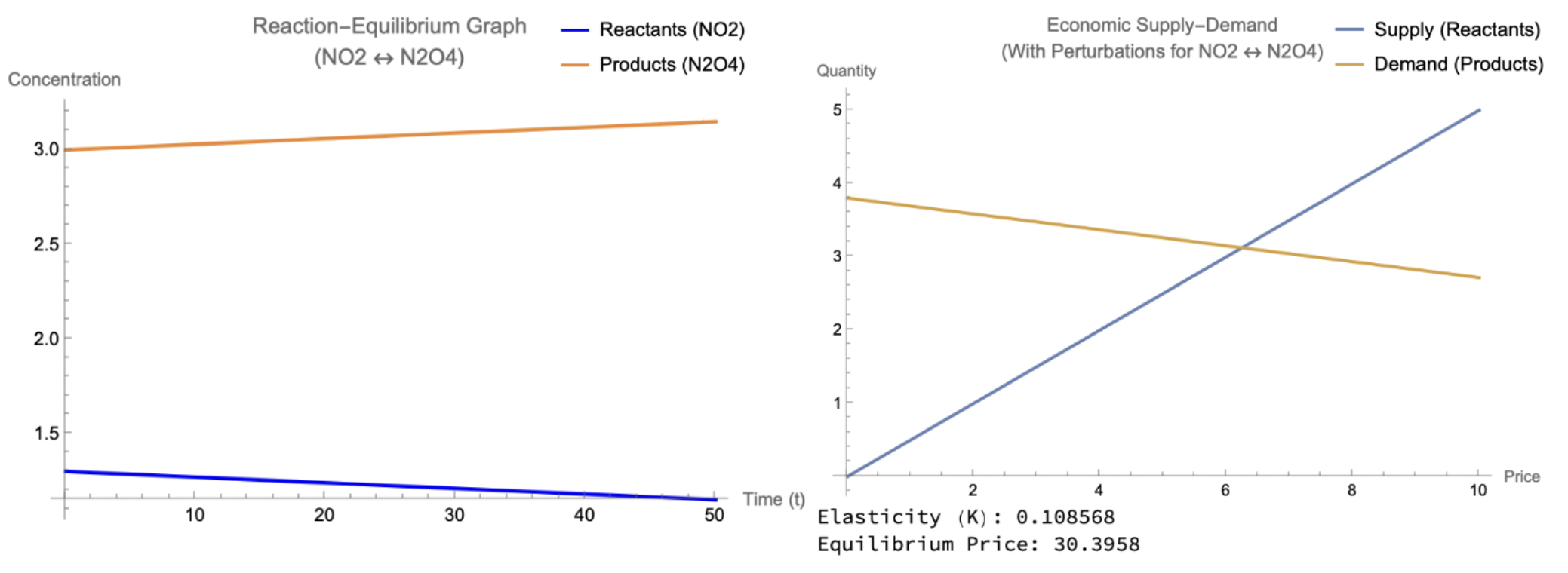
Figure 8:Artificial Equilibrium Compared Between Chemical and Economic Systems
Discussion
The results of this study demonstrate how the fundamental principles of chemical equilibrium and economic supply-demand systems can intersect to model dynamic shifts. Their shifts’ implications were seen in both physical and market environments, adjusting to perturbations and imbalance between reactants and products. When the system began without any products, concentrations steadily decreased while concentrations rose until the equilibrium was reached. This dynamic mirrors real-world markets, as portrayed through the economic markets in the results section. When raw materials are consumed to produce goods, the supply and demand forces successfully stabilize process over time. Additionally, lower elasticities coinciding with higher equilibrium prices tend to occur in resource-dependent markets where the supply is limited, as seen in Figure 7.
Beyond the changes in reactants and products, the models created reveal the significant impact of external perturbations over time. When the reactant concentration was significantly increased (artificially), the reaction shifted to favor the formation of the products, as explained through Le Chatelier’s principle. Similarly, in an economics scenario, this can be compared to a surge in resource availability, where increases and supply can decrease the equilibrium prices. When the opposite occurred in Figure 7, products were artificially manipulated instead of reactants, the system rebalanced to restore equilibrium. This scenario may resemble how excess goods in a market lower demand and alter unique equilibrium conditions.
For future research, extending the model to include temperature and pressure effects on chemical equilibrium may provide deeper insights into additional thermodynamic factors influence on market dynamics. For instance, by directly incorporating temperature as a variable, larger-scale external shocks, such as global events or policy changes, could be simulated to alter certain market conditions. Additionally, an improved model could include real-world data that would adjust for factors such as fluctuating raw material costs or supply chain disruptions, which can enhance the practicality of the model. Lastly, from a chemistry standpoint, more complex reversible reactions may be used to improve certain specifics in the chemistry-economics analogy.
Significance and Implications
By nature, the economics and chemistry fields revolve around systems that are constantly fluctuating. Through cross-discipline exploration, uniting these two fields further highlights the similarities and patterns that can be found in seemingly “random” changes. Many real-world challenges with multifaceted backgrounds align with this background and require a solution that surpasses disciplinary boundaries. For instance, in fields such as environmental economics, a pure economic lens falls short in understanding the balance that must be achieved between natural resources and economic demand—a conclusion that can easily be reached through the integration of chemistry and economics. While chemistry plays a crucial role in managing the use and conservation of resources, economics proposes strategies to allocate these resources efficiently. By combining these fields, researchers can pave the way towards sustainable economic practices, spearheading better strategies for resource management.
Beyond environmental economics, overlaps between economics and chemistry can be seen in upcoming fields, such as energy economics and pharmaceutical industries. By analyzing changes in certain chemical processes —such as carbon emissions— and their influence on economic markets, insights regarding climate change policy and sustainability strategies may also be explored. From an economics lens, because scarcity drives innovation in goods and services, scientists can further contextualize the impacts of chemical innovation on various economic sectors. This may lead to breakthroughs in energy sources and methods of chemical production, creating efficient technologies to maintain and sustain energy-dependent industries.
The heightened focus on the field of green chemistry also holds great promise for economic modeling. Understanding the economic impacts of adopting sustainable technologies may promote and encourage faster acceptance and implementation of sustainable development, such as renewable energy resources. Ultimately, by prioritizing both chemistry and economics perspectives, scientists can drive the transition towards environmentally responsible and economically friendly solutions.
Conclusion
Ultimately, the results of this paper strengthen the interconnectedness between chemical and economic systems. As seen in the models generated, equilibrium, elasticity, and stability have the ability to describe and predict molecular behavior and market dynamics. The low elasticity in various scenarios created in the reaction implies the limited responsiveness to changes in both, chemical models and economic models. As seen in larger industries with higher fixed costs or inflexible supply chains, adapting to attain equilibrium from all viewpoints may prove difficult at certain times. Regardless, this study has explored how abstract science concepts can apply to real-world scenarios, and opens doors for additional interdisciplinary approaches to further strengthen the relation between modeling economic systems using chemical analogies.
The author thanks Mr. Robert Gotwals for assistance with this work. Appreciation is also extended to the Burroughs Wellcome Fund and the North Carolina Science, Mathematics and Technology Center for their funding support for the North Carolina High School Computational Chemistry Server.
Copyright © 2024 Goel. This is an open-access article distributed under the terms of the Creative Commons Attribution 4.0 International license, which enables reusers to distribute, remix, adapt, and build upon the material in any medium or format, so long as attribution is given to the creator.
- DFT
- Density Functional Theory
- Shaymardanov, Z., Shaymardanova, B., Kulenova, N. A., Sadenova, M. A., Shushkevich, L. V., Charykov, N. A., Semenov, K. N., Keskinov, V. A., Blokhin, A. A., Letenko, D. G., Kuznetsov, V. V., & Sadowski, V. (2022). Approach for the Description of Chemical Equilibrium Shifts in the Systems with Free and Connected Chemical Reactions. Processes, 10(12), 2493. 10.3390/pr10122493
- Middelburg, J. J. (2024). The Gibbs Free Energy. In Thermodynamics and Equilibria in Earth System Sciences: An Introduction (pp. 35–46). Springer Nature Switzerland. 10.1007/978-3-031-53407-2_4
- Peris, M. (2021). Understanding Le Châtelier’s principle fundamentals: five key questions. Chemistry Teacher International, 4(3), 203–205. 10.1515/cti-2020-0030
- Perkis, D. F. (2021). The Science of Supply and Demand. https://www.stlouisfed.org/publications/page-one-economics/2021/03/01/the-science-of-supply-and-demand
- Jordan-Wood, S. (2024). Price Elasticity (Demand) Explained. https://www.stlouisfed.org/open-vault/2024/june/price-elasticity-demand-explained
- Farrell, B. F., & Ioannou, P. J. (2000). Perturbation dynamics in atmospheric chemistry. Journal of Geophysical Research: Atmospheres, 105(D7), 9303–9320. 10.1029/1999jd901021
- Romero, M. F., & Rossano, A. J. (2019). Acid-Base Basics. Seminars in Nephrology, 39(4), 316–327. 10.1016/j.semnephrol.2019.04.002
- Schmidt, J. R. ; P. W. F. (2007). WebMo Pro, version 7.0. http://www.webmo.net
- The North Carolina High School Computational Chemistry Server. (2024). http://chemistry.ncssm.edu
- Gaussian. (2024). http://www.gaussian.com