Analyzing Carbon-13 NMR Spectra to Predict Chemical Shifts of Carbon Compounds using Machine Learning Algorithms
Abstract
Nuclear Magnetic Resonance (NMR) is a fundamental tool in chemistry for elucidating the molecular structure of unidentified substances. The evaluation of 13C NMR spectra can be challenging due to the numerous factors that affect the peaks and their locations (chemical shifts). Chemists can use NMR spectroscopy in synthesizing new molecules to confirm the identity of the molecule produced. Since the NMR spectrum for the molecule does not exist, the chemists cannot compare their spectra with preexisting spectra to verify their results. To address this, an algorithm that predicts the chemical shifts of the 13C NMR spectra for compounds based on their molecular structure emerges as a solution, generating artificial spectra for comparison with real ones. This paper delineates a method to formulate such an algorithm using machine learning techniques. Multiple graph neural networks and a classical neural network underwent training on an NMR database to predict the chemical shifts of the 13C NMR spectra for several molecules. The accuracy of each neural network was tested by analyzing the difference between the predictions and the actual chemical shift values in the database using Mean Absolute Error (MAE). Notably, the graph neural networks had a higher accuracy and precision than the classical neural network. Among them, the Graph Transformer Network emerges as the most proficient performer. Chemists can utilize the Graph Transformer Network model to validate the synthesis of new compounds within a margin of error of approximately 2.599 ppm.
Introduction
Nuclear magnetic resonance (NMR) spectroscopy is an effective technique to deduce the molecular structure of a chemical compound. The NMR machine produces a spectrum that can be used in the process of structure elucidation. To predict the molecular structure, the relevant spectral features of the graph, such as the peak locations (chemical shifts), splitting pattern of the peaks, and the integration of the peaks, must be extracted and analyzed GEROTHANASSIS et al., 2002. Interpreting the meaning behind the spectral features of the graph can help determine the structure of the molecule as the spectral features are affected by electron deshielding from electronegative atoms, magnetic anisotropy from pi bonds, and hydrogen bonding GEROTHANASSIS et al., 2002. However, the process of unraveling the spectral features of the NMR spectra based on the molecular structure of the sample can be complex as there are many factors that affect the peaks of the NMR spectra. Machine learning algorithms can be used to predict the spectral features of the NMR spectra of an organic compound based on its chemical structure Kwon et al., 2020. The algorithm would learn the relationship between atoms and bonds in a molecule, and how it affects the NMR spectra of that molecule. Simple neural network algorithms simplify molecules by encapsulating each atom’s features within a vector, albeit at the cost of losing significant information about interatomic interactions. However, a more effective approach to representing molecules for machine learning algorithms emerges with the utilization of graphs Kwon et al., 2020. The graph is composed of nodes, which represent the atoms, that are connected by edges, which represent the bonds between atoms. A graph neural network is a machine learning algorithm that can be used to simulate a compound by mapping out the molecular structure of the compound on a graph. Furthermore, they can be used to predict the chemical shifts of 13C NMR spectra for carbon compounds more accurately than a classic neural network Kwon et al., 2020. The graph neural network algorithm can help scientists while they are producing a new compound as they could use the algorithm to verify if they made the correct compound. Previous studies have shown that graph neural networks are effective in predicting the chemical shifts of 13C NMR spectra Kwon et al., 2020. In this study, I aim to further improve the accuracy of the graph neural networks by introducing novel architectural frameworks that incorporate comprehensive data from both nodes and edges within each graph. The algorithm is tested by comparing the actual chemical shift values of 13C NMR spectra with the predicted chemical shift values from the algorithm for various carbon compounds. The actual chemical shift values of the 13C NMR spectra is obtained from the NMRShiftDb2 database.
Methods
Data Preprocessing
The dataset used in this paper is the NMRShiftDB2 database, which contains the NMR spectra data for 17,473 unique molecules. Some molecules have spectral data for 13C NMR spectra, other molecules have spectral data for 1H NMR spectra, while the rest of them have spectral data for both 13C NMR and 1H NMR spectra. Since I am only analyzing 13C NMR spectra, I went through the database and removed the molecules that do not have data for 13C NMR spectra. Only 7,304 molecules in the dataset had data for 13C NMR spectra.
Table 1:Node features
| Node Feature | Data Type |
|---|---|
| Atomic Number | Integer (1-118) |
| Number of Neighbors | Integer |
| Formal Charge | Integer |
| Hybridization | One-hot encoded (, , , , ) |
| Aromaticity | One-hot encoded (yes, no) |
| Total Numer of Hydrogens | Integer |
| Number of Radical Electrons | Integer |
| In Ring | One-hot encoded (yes, no) |
| Chirality | One-hot encoded (clockwise, counterclockwise, no) |
Table 2:Edge Features
| Edge Feature | Data Type |
|---|---|
| Bond Type | One-hot encoded (single, aromatic, double) |
| In Ring | One-hot encoded (yes, no) |
| Is Conjugated | One-hot encoded (yes, no) |
Each molecule in the dataset is represented as a graph to be used by the different graph neural networks. The nodes of a graph represent the different atoms in a molecule and the edges of a graph represent the bonds between each atom in a molecule. Let represent an edge of a graph where represents the initial node and represents the terminal node. Since the bonds in a molecule are undirected, the edges in the graph are also undirected, so . I went through each bond in the molecule and noted the indices of the atom in the bond using two arrays and combined them in one array in the format, [[i, j], [j, i]]. The edge indices are extracted using the RDKit Python library by using the SMILES string of each molecule. The SMILES string encodes the molecular structure of a compound in a string object for the computer to read it. I combined all the edge indices in one matrix and stored it in a torch.Tensor object using the PyTorch Geometric Python library.
Let represent a node in a graph. Each node in a graph has nine node features stored in a array. The different node features can be shown in Table 1. All the node features are extracted using the RDKit Python library by using the SMILES string of each molecule. The different node feature arrays for each graph are combined into a multidimensional matrix torch.Tensor object using the PyTorch Geometric Python library. Let represent the multidimensional matrix whose dimensions are the . The matrix contains all the node features in a molecule such that .

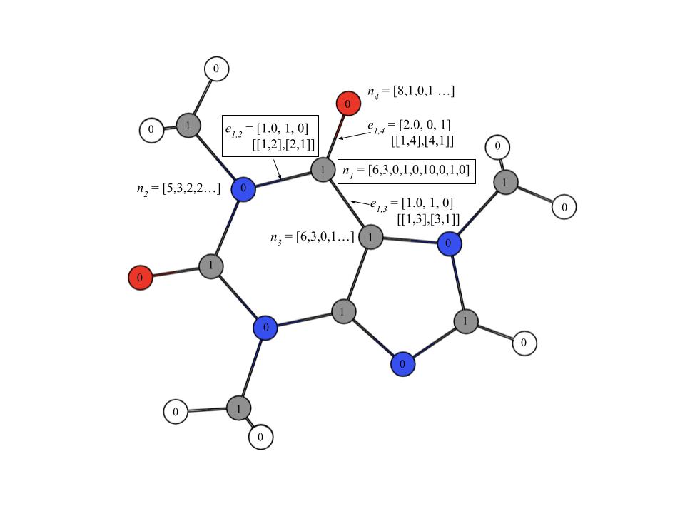
Figure 1:Example of a Molecular Graph
In Figure 1 the selected node illustrates an example of a node feature array with nine elements. The elements refer to the features in Table 1. The selected edge shows an example of an edge feature array with three elements and an adjacency list with two arrays. The elements in the edge feature array refer to the features in Table 2. There are two arrays for every edge as they are undirected. Each node is labeled with a 0 or 1, where 0 represents the node is not carbon and 1 represents the node is carbon. The binary values are stored in the mask array.
Let represent an edge in a graph. Each edge in a graph has three edge features stored in a array. The different edge features can be shown in Table 2. All the edge features are extracted using the RDKit Python library by using the SMILES string of each molecule. The different edge feature arrays for each graph are combined into a multidimensional matrix torch.Tensor object using the PyTorch Geometric Python library. Let represent the multidimensional matrix whose dimensions are the . The matrix contains all the edge features in a molecule such that .
While going through the atoms in the molecule, I stored the atom indices of carbon atoms in an array where the integer 1 indicated that the atom is carbon and the integer 0 indicated that the atom is not carbon. These arrays are called masks and it helps the graph neural networks to identify the nodes that represent the NMR-active atoms in a molecule. The mask array is stored in a torch.Tensor object. Let m represent the mask array whose dimensions are the . After obtaining all the torch.Tensor objects for a molecule, I created an object for each graph that combined the torch.Tensor objects for node features, edge features, edge indices, and masks to be used as input for the graph neural networks. Figure 1 shows an example of how the molecules are encoded into graphs where each node and edge represent the atoms and bonds respectively, and each node is labeled with a binary mask to determine whether an atom is carbon or not.
Graph Neural Networks
To predict the chemical shifts of 13C NMR spectra for carbon compounds, I utilized several different types of graph neural networks. The graph neural networks take in the graphs of the different molecules as the input and output an array of the predicted chemical shifts with size for each molecule. The neural networks used Mean Absolute Error (MAE) to calculate the loss for the chemical shifts by subtracting the predicted chemical shifts with the actual chemical shifts and taking the absolute value of the difference. Then, the neural networks find the average error of all the chemical shifts for every molecule in a set. The following equation describes how MAE is calculated:
where is a set of molecules, is a molecule in the set , is the actual chemical shift of one atom in the molecule , and is the predicted chemical shift for that one atom. After each layer in the graph neural networks, a layer normalization, dropout, and ReLU function is applied to the data, respectively. The layer normalization transforms the data to be on a similar scale and is used to stabilize and speed up the training process Ba et al., 2016. The dropout function randomly ignores a certain number of nodes in the next layer to prevent overfitting in the graph neural network Srivastava et al., 2014. The ReLU function ensures nonlinearity and prevents the gradients in the graph neural networks from becoming too small by removing negative values in the data.
Graph Transformer Network
One of the graph neural networks used was a Graph Transformer Network. The Graph Transformer Network is a specific type of graph neural network that updates the node features of one node based on the features of its neighboring nodes. The neural network performs an aggregation function that combines the node features of one node with the node features of its neighboring nodes. For the Graph Transformer Network used in this paper, I took the sum of the node features of the neighboring nodes. Along with the aggregation function, the Graph Transformer Network uses a self-attention mechanism that performs a dot product with the neighboring node features to determine which of the neighboring nodes are important for the chemical shift prediction. The weights for the self-attention mechanism is learnable and it gets updated as the Graph Transformer Network is training. In addition to the aggregation function and self-attention mechanism, the Graph Transformer Network multiplies more learnable weights to the node being updated and its neighboring nodes.
The following equation shows how the Graph Transformer Network updates each node in a graph Fey & Lenssen, 2019:
where is the node before being updated, is the neighboring nodes, is the self-attention mechanism, and & are the learnable weights multiplied to each node. The Graph Transformer Network determines the learnable self-attention mechanism using the following function Fey & Lenssen, 2019:
where is the node before being updated, is a neighboring node, and & are the learnable weights multiplied to each node in the self-attention mechanism. The softmax function normalizes the self-attention mechanisms from all the neighboring nodes to have a sum of 1. The self-attention mechanism divides by inside the softmax function to maintain a standard normal distribution by keeping a variance of 1 and mean of 0.
Graph Attention Network
One of the other graph neural networks used in this paper is the Graph Attention Network. The Graph Attention Network is similar to the Graph Transformer Network, except that it uses different functions (Equations (4) & (5)) to update each node and calculate the self-attention mechanisms.
The Graph Attention Network uses the following function to update each node in the graph Fey & Lenssen, 2019:
where the learnable weights are the same throughout the entire function instead of the function for the Graph Transformer Network that uses two different learnable weights. The Graph Attention Network also applies a dot product to the self-attention mechanism and the node being updated.
The Graph Attention Network uses the following function to calculate the self-attention mechanism Fey & Lenssen, 2019:
where is the edge feature of the edge connecting nodes and , is the learnable weights for the edge features, and is the learnable attention vector that determines the weight of each neighboring node. The LeakyReLU function has the same functionality as the ReLU function, but allows for negative values at a low magnitude Xu et al., 2015. The function is used to normalize the self-attention mechanisms instead of the softmax function in the Graph Transformer Network, and gets rid of negative values. The operation in the function concatenates the three arrays.
Graph Convolution Network
The last graph neural network used in this paper is the Graph Convolutional Network (GCN). The GCN is different from the Graph Attention Network and Graph Transformer Network as it does not have a self-attention mechanism and uses a different function to update the nodes in a graph. The GCN updates nodes in the graph using the following function Fey & Lenssen, 2019:
where
where is the edge feature of the edge connecting nodes and . The GCN only uses the edge features in the graph and does not consider the features of the neighboring nodes. The GCN is less complex than the Graph Attention Network and Graph Transformer Network as it uses less data from the graph and only has one set of learnable weights.
Training, Validation, and Testing
The training, validation, and testing of the graph neural networks were performed by splitting the dataset into 80, 10, and 10 percent for the training, validation, and test sets, respectively. Then, the training, validation, and test sets were split into equal size batches for the graph neural networks to be trained faster. The graph neural networks went through one hundred epochs during the training process, where each epoch iterated through the entire training set once. In order to ensure that the loss was decreasing, at the end of each epoch, the graph neural networks went through the validation set and printed the average loss from the validation set using MAE. At the end of the one hundred epochs, the graph neural networks went through the test set and printed the average loss from the test set using MAE to determine the performance of each graph neural network.
Results and Discussion
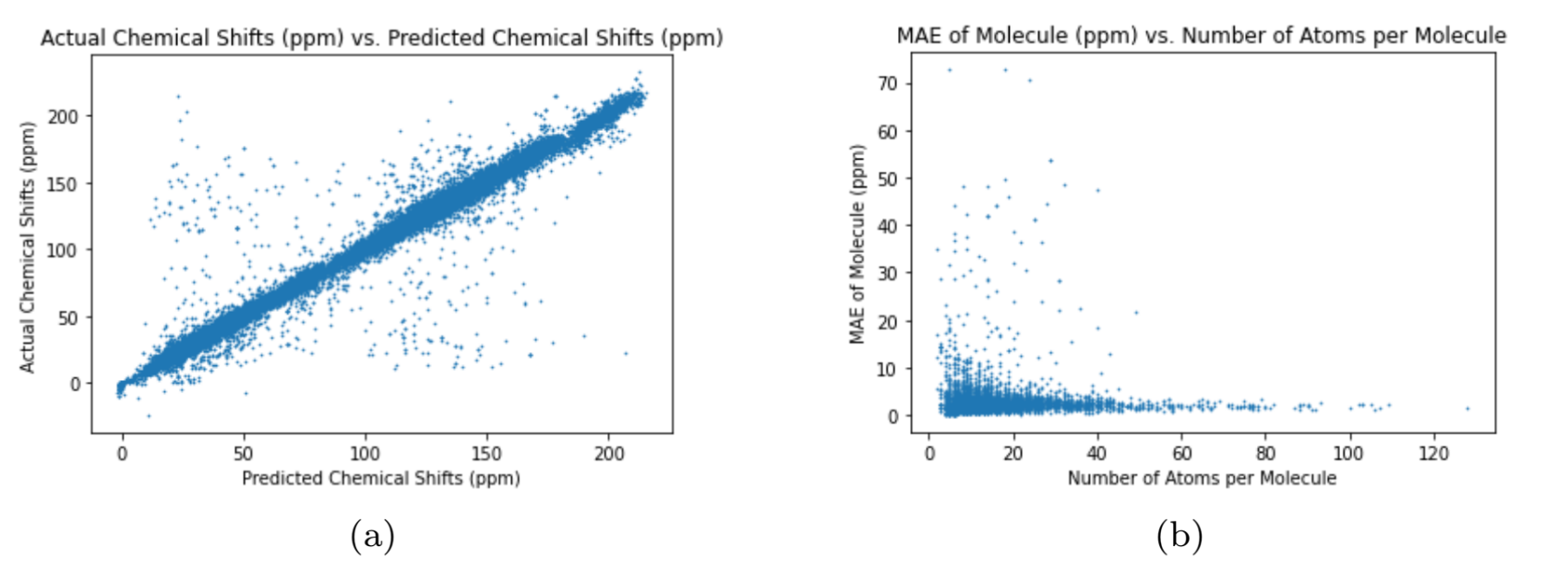
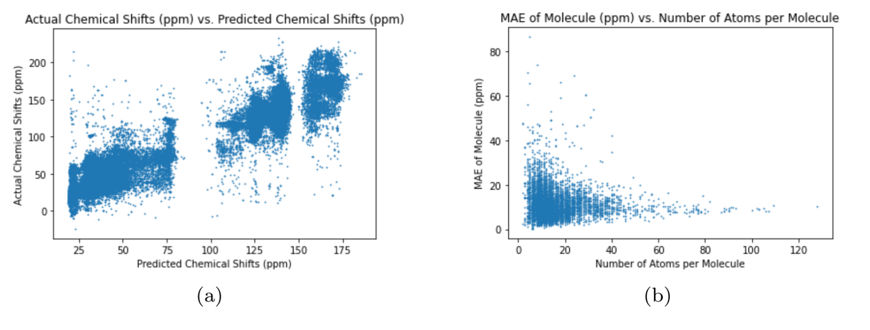
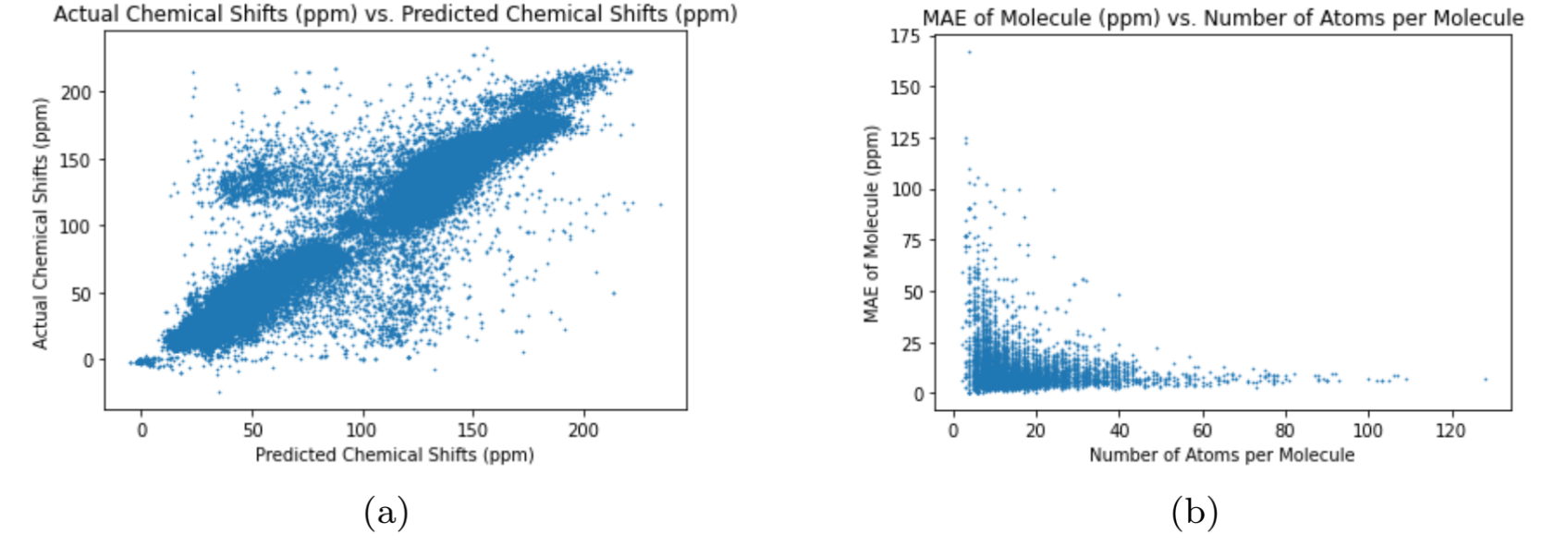
The different graph neural networks were tested several times to determine the graph neural network with the best performance. The Multi-Layer Perceptron (MLP) is a classical neural network model that does not use graphs as input Murtagh, 1991. I used the MLP as a benchmark test for the other graph neural networks to compare the performance of graph neural networks with regular neural networks. To assess the neural networks, I ran each neural network 10 times through the training, validation, and test cycle. In each trial, I randomized the seed for weight initialization to obtain a range of values for the test loss using MAE (Equation (1)). The results of each neural network can be seen in Table 3. The test loss values for each neural network represents the average test loss over the 10 trials, plus or minus the standard deviation. The results show that the Graph Transformer Network has the best performance compared to the other neural networks. The average test loss for the Graph Transformer Network was 2.599 ppm, which is not better than the existing graph neural networks from previous works but is close Kwon et al., 2020. The loss is significantly low as the 13C NMR spectra has chemical shift values ranging from 0 ppm to 220 ppm. The other graph neural networks passed the benchmark test by having lower average test losses than the Multi-Layer Perceptron neural network. This proves that graph neural networks are superior to classic neural networks in predicting the chemical shifts of 13C NMR spectra for carbon compounds. The difference in test loss between the Graph Convolutional Network and the other two graph neural networks shows that the self-attention mechanisms greatly improve the performance of the graph neural networks. The increased accuracy of the Graph Transformer Network over the Graph Attention Network reveals that using more sets of learnable weights improves the performance of the graph neural network. The plots in 2, 3, 4, and 5 further demonstrate the performance of the Graph Transformer Network over the other neural networks for predicting the chemical shifts of 13C NMR spectra (2, 3, 4, and 5).

Figure 2:Performance of Graph Transformer Network

Figure 3:Performance of Multi-Layer Perceptron

Figure 4:Performance of Graph Convolutional Network

Figure 5:Performance of Graph Attention Network
For plot (a) in 2, 3, 4, and 5, the neural network is more accurate if the data is closer to the line, (2, 3, 4, and 5). The Graph Transformer Network is the most accurate while the Multi-Layer Perceptron is the least accurate. Also, the Graph Attention Network is more accurate than the Graph Convolutional Network. The variance of the data in the plots in 2, 3, 4, and 5 reveal the preciseness of eachneural network (2, 3, 4, and 5). The Graph Transformer Network is the most precise with 2.74% of its data being outliers, and the Multi-Layer Perceptron is the least precise with 39.98% of its data being outliers. The Graph Attention Network is more precise than the Graph Convolutional Network as 11.91% of the data from the Graph Attention Network are outliers and 31.76% of the data from the Graph Convolutional Network are outliers. The test loss numbers in Table 3 explains the pattern above as the Graph Transformer Network has the lowest test loss and the Multi-Layer Perceptron has the highest test loss. The plot (b) in 2, 3, 4, and 5 shows the accuracy of the neural networks for predicting the chemical shifts of 13C NMR spectra for molecules with varying 8 amounts of atoms (2, 3, 4, and 5). The plot shows that the neural networks can more accurately predict the chemical shift values of 13C NMR spectra for molecules containing more atoms. This is due to the increase in data for each molecule as the atoms increase, causing the neural networks to produce more accurate predictions.
Table 3:Performance of Neural Networks
| Neural Network | Test Loss (ppm) |
|---|---|
| Graph Transformer Network | 2.599 ± 0.3169 |
| Multi-Layer Perceptron | 9.152 ± 2.543 |
| Graph Convolutional Network | 8.639 ± 1.619 |
| Graph Attention Network | 4.488 ± 1.379 |
Conclusion
In this study, I predicted the chemical shifts of 13C NMR spectra for carbon compounds using neural networks aiming to assist chemists with confirming the synthesis of new compounds. Leveraging a database of molecules with the chemical shifts of their associated 13C NMR spectra, I trained and tested the neural networks. These encompassed three different types of graph neural networks and a classical neural network to test whether the graph neural networks can perform better than the classical neural network. I encoded each molecule in a graph, where the nodes are the atoms of the molecules and the edges are the bonds between the atoms, as input for the graph neural networks. I used MAE to evaluate the performance of each neural network. The Graph Transformer Network had a MAE of 2.599 ppm, the Multi-Layer Perceptron had a MAE of 9.152 ppm, the Graph Convolutional Network had a MAE of 8.639 ppm, and the Graph Attention Network had a MAE of 4.488 ppm. The Graph Transformer Network had the best accuracy for predicting the chemical shifts and all three of the graph neural networks performed better than the classical neural network.
The performance of the Graph Transformer Network is not superior but is close to the performance of existing methods, which has a MAE of 1.355 ppm Kwon et al., 2020. The model for the Graph Transformer Network can be used by chemists for verifying the synthesization of new molecules. The performance of the neural networks can be improved by training them with a larger database. For future work, I can test the algorithm for predicting the chemical shifts of other types of NMR spectra and improve the performance of the graph neural by utilizing different architectures.
Copyright © 2024 Agrawala. This is an open-access article distributed under the terms of the Creative Commons Attribution 4.0 International license, which enables reusers to distribute, remix, adapt, and build upon the material in any medium or format, so long as attribution is given to the creator.
- GCN
- Graph Convolutional Network
- MAE
- Mean Absolute Error
- MLP
- Multi-Layer Perceptron
- NMR
- Nuclear Magnetic Resonance
- GEROTHANASSIS, I. P., TROGANIS, A., EXARCHOU, V., & BARBAROSSOU, K. (2002). NUCLEAR MAGNETIC RESONANCE (NMR) SPECTROSCOPY: BASIC PRINCIPLES AND PHENOMENA, AND THEIR APPLICATIONS TO CHEMISTRY, BIOLOGY AND MEDICINE. Chem. Educ. Res. Pract., 3(2), 229–252. 10.1039/b2rp90018a
- Kwon, Y., Lee, D., Choi, Y.-S., Kang, M., & Kang, S. (2020). Neural Message Passing for NMR Chemical Shift Prediction. Journal of Chemical Information and Modeling, 60(4), 2024–2030. 10.1021/acs.jcim.0c00195
- Ba, J. L., Kiros, J. R., & Hinton, G. E. (2016). Layer Normalization. arXiv. 10.48550/ARXIV.1607.06450
- Srivastava, N., Hinton, G., Krizhevsky, A., Sutskever, I., & Salakhutdinov, R. (2014). Dropout: A Simple Way to Prevent Neural Networks from Overfitting. Journal of Machine Learning Research, 15(56), 1929–1958. http://jmlr.org/papers/v15/srivastava14a.html
- Fey, M., & Lenssen, J. E. (2019). Fast Graph Representation Learning with PyTorch Geometric. arXiv. 10.48550/ARXIV.1903.02428
- Xu, B., Wang, N., Chen, T., & Li, M. (2015). Empirical Evaluation of Rectified Activations in Convolutional Network. arXiv. 10.48550/ARXIV.1505.00853
- Murtagh, F. (1991). Multilayer perceptrons for classification and regression. Neurocomputing, 2(5–6), 183–197. 10.1016/0925-2312(91)90023-5
