AQINet: A multimodal deep convolutional neural network to predict Air Quality Index via satellite imagery and meteorological data
Abstract
Air pollution is a pressing ecological issue with significant impacts on both public health and the environment. Poor air quality is a major contributor to respiratory diseases and is linked to millions of deaths annually, but many countries cannot afford air monitoring equipment. This lack of data makes it difficult to assess the health and environmental risks resulting from pollutant exposure. To address this problem, we present a multimodal model to inexpensively predict air quality levels in densely populated areas. Our research leverages both satellite imagery and meteorological data to create accurate air quality predictions. We sourced urban and suburban satellite imagery from the National Agriculture Imaging Program, meteorological data from Open-Meteo, and air quality data from OpenWeatherMap, to create a dataset named AQISet. AQISet is publicly available and free to download. The goal was for the model to implicitly learn spatial features in each image, such as roads, greenery, and bodies of water, and then combine this info with meteorological data to predict AQI. Using multiple computer vision techniques, the model was able to predict AQI with a mean absolute error of 16 AQI and a classification accuracy of 77% based on the EPA’s AQI standards categories. Our results establish a baseline for AQI prediction from satellite imagery and are a vast improvement over state-of-the-art pre-trained general computer vision models.
Introduction
The process of respiration is essential for all living organisms, as it enables them to produce energy. Consequently, access to clean air is fundamental for life to be sustained. Exposure to air pollution can lead to a multitude of health issues such as respiratory ailments, cardiovascular diseases, and in severe cases, death U.S. EPA, 2017.
Despite concerted global efforts to mitigate air pollution in recent decades, a startling statistic from 2019 shows that 99% of the world’s population resides in areas that fail to meet the World Health Organization’s air quality standards Ambient (outdoor) air pollution, n.d.. This alarming situation has led to over 4 million deaths annually, predominantly in low and middle-income countries, which account for 89% of these fatalities linked to ambient air pollution.
Air Quality Index (AQI), a metric of air pollution developed by the United States Environmental Protection Agency (EPA), quantifies air pollution levels AQI Basics | AirNow.gov, n.d.. AQI is computed based on measurements of several pollutants, chiefly particulate matter (PM2.5 and PM10), nitrogen dioxide (NO2), ozone (O3), carbon monoxide (CO), and sulfur dioxide (SO2). These pollutants arise from a variety of sources such as man-made emissions from fossil fuels, as well as natural sources like smoke from volcanoes and wildfires.
Ground-based air quality monitors are typically used to measure the concentration of each pollutant over a certain time frame. These devices vary in size, from small household units to medium and large static monitors strategically positioned around cities, offering continuous data from selected urban locations. These types of sensors utilize active measurement techniques, which use physical or chemical methods to analyze the air in a given area automatically. These sensors can be extremely expensive to manufacture and operate, and costs can range from 15,000 dollars to 40,000 dollars per sensor U.S. EPA, 2019. This high cost poses a onsiderable challenge to lesser developed regions of the world where governments may struggle to afford many air quality monitors to monitor urban and suburban areas adequately. According to the United Nations International Children’s Emergency Fund (UNICEF), only about 6% and 24% of children live within 50km of an air quality monitor in Africa and South America respectively UNICEF, 2019. The lack of AQI data in developing countries can lead to unnecessary pollutant exposure and affect regulatory processes, as authorities struggle to assess pollution levels and take appropriate actions.
Table 1:Health Risks of Air Pollutants
| Pollutant | Health Risks |
|---|---|
| Particulate Matter | Irritation of airways, aggravated asthma, and lung cancer. |
| NO2 | Inflammation of airways, worsened cough reduced lung function, and increased asthma attacks. |
| O3 | Chest pain, coughing, throat irritation, and congestion. |
| CO | Headache, nausea, rapid breathing, dizziness, and confusion. |
| SO2 | Irritation of eyes, nose, throat, and airways, and aggravation of asthma and emphysema. |
Previous Work
Other scientists have conducted experiments using satellite data to predict air pollution levels in certain areas. Scheibenreif et al. used imagery and remote sensing measurements from the European Space Agency’s Sentinel satellites and a two-stream deep neural network to predict levels of nitrogen dioxide, one of the major pollutants in computing the AQI Scheibenreif et al., 2022. Rowley et. al built off of this approach and used the Sentinel satellites along with NO2 ground monitoring stations to predict levels of NO2, O3, and PM10 Rowley & Karakuş, 2022. They also included a fully connected neural network that utilized additional data such as population and altitude. This project aims to provide a more general prediction of air quality by directly predicting the AQI rather than the pollutants that comprise it.
Dataset Creation
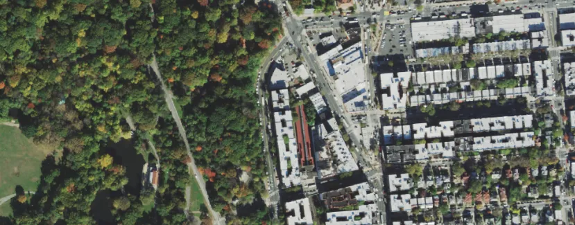
At the time this research was conducted, there were no publicly available datasets that included satellite imagery with time, location, AQI, and meteorological data. To train our model, we compiled our own dataset, AQISet, by retrieving data from different sources Sihorwala, n.d.. We started by collecting the most inflexible of the three, satellite imagery. Since 2002, the US Department of Agriculture has operated the National Agriculture Imagery Program (NAIP), which collects high-resolution imagery across the United States from urban and suburban regions National Agriculture Imagery Program - NAIP Hub Site, n.d.. This data is accessible through Google Earth Engine, a geospatial analysis program that allows users to write Python code to export imagery Google Earth Engine, n.d.. We gathered longitude and latitude data for the 100 largest cities in America and then wrote a script to collect 100 1km by 1km images from each city, each with 1m per pixel resolution. We utilized 25 parallel processes to export all of the imagery. Since the NAIP dataset did not have complete coverage of all the areas we targeted, only 7,621 images were gathered out of an attempted 10,000, but this amount was still suitable for our dataset and model. A sample image is below:

Figure 1:A sample satellite image in AQISet.
Alongside the imagery, we also collected the time and location of capture for each image so that we could use the timestamp and coordinates of the images to pair them up with AQI and meteorological data. The air quality data was retrieved from OpenWeatherMap, a service that provides global weather and environmental data via API calls. Current weather and forecast - OpenWeatherMap, n.d.. However, OpenWeatherMap provides pollutant concentrations rather than directly providing AQI values, so we converted the concentrations to AQI in the data preprocessing. The first step was to convert the units of each pollutant from μg/m3 to ppb Danish National Environmental Research Institute, n.d.. The equation is as follows:
Where M is the molecular weight of the pollutant and C is the surface temperature in ◦C. Then, we converted these concentrations to an AQI value using an equation and a table of breakpoints provided by the EPA Air quality index, 2024. The equation is as follows AirNow, n.d.:
Where C is the pollutant concentration, Chi is the concentration breakpoint greater than or equal to equal to C, Clo is the breakpoint less than or equal to C, and Chi and Clo are the corresponding AQI breakpoints of Chi and Clo respectively.
Finally, the overall AQI is simply the maximum AQI calculated for each pollutant. These AQI values were paired with each image based on time and location. For our meteorological data, we collected four different factors: wind speed, humidity, temperature, and rain. Rain was further split up into 3 categories, a sum of precipitation over 24 hours, 8 hours, and 1 hour. A table of their respective effects on AQI is below.
Table 2:Effects of Meteorological Factors on AQI
| Weather Factor | Effects on AQI |
|---|---|
| Rain | Rain can wash away particulate matter, cleansing the air. |
| Temperature | Higher temperatures accelerate photochemical reactions, resulting in more ground level O3 |
| Humidity | Water vapor can serve as nuclei for small particles, which can result in the formation of larger particulates. |
| Wind Speed | Higher wind speeds can disperse pollutants by blowing them away. |
This data was retrieved via API calls to Open-Meteo Open-Meteo, n.d., a meteorological data service, and then paired up with each image in a similar manner to the AQI data.
Materials
The model was built in Python 3.11.4 using the PyTorch library for machine learning. All of the data was processed using the Pandas library. Smaller testing of the model (less than 5 epochs) was conducted on Michigan State University’s (MSU) CVLab GPU server, using 4 Titan V GPUs. Larger tests were run using an NVIDIA V100 Tensor Core GPU from MSU’s High Power Computing Center with the UNIX command-line interface. The model uses a learning rate of 0.001 and a batch size of 64 images.
Methods
Our model is split into two parts: the image network and the tabular network. The basis of our image network is ResNet-50, a 50-layer convolutional neural network pre-trained for image classification tasks He et al., 2015. Although our problem is fundamentally that of regression, the main goal of the image network is to implicitly learn certain features of an image to produce an accurate prediction such as the amount of greenery, roads, cars, buildings, and bodies of water present. These can all affect the overall AQI of an area, and it is crucial to use a deep network so that it is able to learn these complex features in the image. We modified ResNet-50 to include an extra channel of input (which will be discussed later) and increased its initial convolution kernel size from 7x7 to 8x8 to help the model capture broader areas of information from the image while decreasing computational complexity. The output from the modified ResNet-50 is then passed through three fully connected layers with Swish activation. We chose to use Swish over other popular activation functions such as Rectified Linear Unit (ReLU) due to Swish’s non-linearity, which allows the model to learn complex relationships between inputs and outputs.
The tabular network is a multilayer perceptron that takes the amount of rain, humidity, temperature, and wind speed as input. These four factors were selected due to their direct effect on and strong correlation with AQI.

Figure 2:R2 values of various meteorological factors and AQI.
The outputs from the image network and the tabular data network are then combined, passed through a few more layers - again with Swish activation - and are eventually narrowed down to a layer with one neuron which holds the AQI prediction.

Figure 3:AQINet model architecture.
In the model above, the larger the block, the greater the amount of neurons in the layer. The blocks decrease in size, effectively narrowing down the data passed through each layer until there is a single neuron left.
Before we trained and tested the AQINet model, we had to resolve a major issue stemming from our dataset: AQI imbalance. AQI values are not evenly distributed in the real world, and this is reflected in our dataset as seen below.

Figure 4:AQI value frequencies in AQISet.
The majority of the AQI values range from 25 to 50 AQI, and this imbalance will lead our model to simply predict from the small range of AQI values that are the most frequent. Consequently, the model will be rewarded for a majority of its predictions, and will not learn. There are two methods we took to approach this.
The first method is using upsampling to even out the AQI distribution by taking more samples of images with infrequent AQIs. Instead of feeding our model the entire 1000px by 1000px image, we take N 224x224 patches from the image. N is proportional to the inverse of our frequency graph so that images with infrequent AQI are sampled much more than those with common AQI, effectively evening out AQI distribution in our data.
The second method we use is a weighted loss function to punish the model more for incorrect guesses on infrequent AQI. We started with a standard Mean Squared Error (MSE) loss, the square of the difference between the model’s prediction and the ground truth AQI. Then, we computed some weight for each AQI, W, to scale our MSE loss by. W is defined as follows:
Where N is a Gaussian kernel with μ mean frequency and σ 2 variance, F is our frequency distribution, and is the ground truth AQI for patch i. The asterisk (∗) in the equation represents a convolution, rather than multiplication. This convolution serves to smooth our frequency distribution so that our weights are calculated based on large changes in the frequency rather than small inconsistencies. This is illustrated in the graph below.

Figure 5:The smoothed AQI frequency distribution.
After computing this weight, the total loss for an image with n patches is simply the sum of the weights multiplied by MSE loss:
In this equation, k is a scalar applied to the function to prevent the loss from becoming very small since often W will be significantly less than 1. A very small loss will adversely affect the training of our model by diminishing the gradients and slowing down the learning. Together both the upsampling and weighted loss solve the issue of data imbalance, and allow the model to predict the full range of AQI values (0-500).
A minor issue with our dataset arises from the limited variance in AQI values at each location from which images were sourced. In each city, the proximity of image capture points—often just a few kilometers apart—resulted in numerous images from nearby areas exhibiting identical AQI values since the data would come from the same sensor. This presents a challenge for our model, as it could lead to overfitting, with the model erroneously predicting specific AQI values that frequently appear in the dataset. To address this, we introduced a range of noise, varying from -5 to +5 AQI, to each patch taken from an image. We used a Gaussian noise distribution across all of the patches, ensuring that the mean AQI across the patches was equivalent to the original AQI. This noise introduction aims to improve our model’s robustness, ensuring better generalization when it inevitably encounters new data in testing.
One discernible feature of poor air quality in images is the haziness or subtle blurring effect caused by dust and other airborne particulates. To capture this trait, we use a 2D Fourier transform to transform our RGB image input into the frequency domain, thereby adding a fourth channel to our image network. The frequency domain is particularly effective in highlighting the haziness of an image since it can reflect it in its low-frequency components. We first converted the RGB image to grayscale by averaging the values from the red, green, and blue input channels. Then, we normalize each pixel value to range from 0-1 rather than 0-255 to improve computational speed. We then treat the pixel values as a stream of numbers, or a signal. This signal is decomposed into sine and cosine waves using the Fast Fourier Transform (FFT). The resulting projected FFT image generally appears darker in areas representing low frequencies, indicative of smooth transitions over time, and brighter in areas with high frequencies, corresponding to finer details in the image. This transformed image is subsequently fed into the model for analysis. Below are a few examples of these transformations.

Figure 6:Imagery and their Fourier transforms. The top image contains haze, which results in a darker frequency domain. The AQI for the top image is 185, while the bottom image’s AQI is 52.
Results

Figure 7:AQI MAE for ResNet-50 vs. AQINet.
In testing, AQINet outperforms ResNet-50 in both Mean Absolute Error and classification accuracy. AQI - more than a 48% improvement. Classification accuracy was based on whether the model could place an image into its corresponding AQI category, based on the EPA’s table of AQI categories AirNow, n.d..

Figure 8:Classification Accuracy for ResNet-50 vs. AQINet.
Conclusion
This research represents a significant step forward in addressing the pressing issue of air pollution and its consequences for public health. By harnessing the power of satellite imagery and meteorological data, the developed multimodal model, AQINet, offers an inexpensive solution for predicting air quality levels in developing areas. This model has shown impressive results, achieving a mean absolute error of 16 AQI (on a scale from 0-500) and a classification accuracy of 77%, based on the EPA’s AQI standards categories.
The ability to predict AQI from satellite imagery has the potential to revolutionize air quality monitoring, especially in regions with limited access to expensive air quality sensors. This approach can provide a cost-effective means of obtaining widespread air quality data, offering substantial benefits for both researchers and policymakers.
Alongside AQINet, we also presented AQISet, a dataset with over 7600 satellite images paired with their AQI and various meteorological data from the time and location of capture. This dataset can help future researchers continue to tackle the issues of air quality monitoring by developing their own models. AQISet is publicly available on GitHub Sihorwala, n.d..
Together, AQINet and AQISet provide a solid foundation for future endeavors in air quality prediction using remote sensing data. Further enhancements and refinements of the model could lead to even more accurate and robust predictions, ultimately contributing to the improvement of air quality and the well-being of communities around the world.
I would like to acknowledge Dr. Xiaoming Liu and Dr. Feng Liu for providing me with a great introduction to computer vision, as well as the rest of the CV Lab for their help during my research.
Copyright © 2024 Sihorwala. This is an open-access article distributed under the terms of the Creative Commons Attribution 4.0 International license, which enables reusers to distribute, remix, adapt, and build upon the material in any medium or format, so long as attribution is given to the creator.
- API
- Application programming interface
- AQI
- Air Quality Index
- EPA
- Environmental Protection Agency
- FFT
- Fast Fourier Transform
- GPU
- Graphics processing unit
- MAE
- Mean Absolute Error
- MSU
- Michigan State University
- NAIP
- The National Agricultural Imagery Program
- ReLU
- Rectified Linear Unit
- RGB
- Red Green Blue
- UNICEF
- United Nations International Children's Emergency Fund
- Trends Report 2003. (2017). U.S. EPA. https://www.epa.gov/sites/default/files/2017-11/documents/trends_report_2003.pdf
- Ambient (outdoor) air pollution. (n.d.). https://www.who.int/news-room/fact-sheets/detail/ambient-(outdoor)-air-quality-and-health
- AQI Basics | AirNow.gov. (n.d.). https://www.airnow.gov/aqi/aqi-basics
- FRM/FEM and Air Sensors. (2019). U.S. EPA. https://www.epa.gov/sites/default/files/2019-12/documents/frm-fem_and_air_sensors_dec_2019_webinar_slides_508_compliant.pdf
- Silent Suffocation in Africa: Air Pollution. (2019). UNICEF. https://www.unicef.org/media/55081/file/Silent%20suffocation%20in%20africa%20air%20pollution%202019%20.pdf
- Scheibenreif, L., Mommert, M., & Borth, D. (2022). Toward Global Estimation of Ground-Level NO ₂ Pollution With Deep Learning and Remote Sensing. IEEE Transactions on Geoscience and Remote Sensing, 60, 1–14. 10.1109/TGRS.2022.3160827
- Rowley, A., & Karakuş, O. (2022). Predicting air quality via multimodal AI and satellite imagery. 10.48550/ARXIV.2211.00780
- Sihorwala, Z. (n.d.). AQISet. https://github.com/zoaibs/AQISet
- National Agriculture Imagery Program - NAIP Hub Site. (n.d.). https://naip-usdaonline.hub.arcgis.com/
- Google Earth Engine. (n.d.). https://earthengine.google.com/
- Current weather and forecast - OpenWeatherMap. (n.d.). https://openweathermap.org/
- Danish National Environmental Research Institute. (n.d.). In Conversion between ppm and μg/m^3.
- Air quality index. (2024). In Wikipedia. https://en.wikipedia.org/w/index.php?title=Air_quality_index&oldid=1221043689
- AQI Technical Assistance Document. (n.d.). AirNow. https://www.airnow.gov/sites/default/files/2020-05/aqi-technical-assistance-document-sept2018.pdf
- Open-Meteo. (n.d.). Open-Meteo. https://open-meteo.com/